Originally published in Towards Data Science

What if I want to know how words have changed over time? For example, I may want to quantify the ways certain words (such as “mask” or “lockdown”) were used before the COVID-19 pandemic and how they evolved through the pandemic. Detecting how and when word usage changed over time can be useful from a linguistic and cultural standpoint as well as from a policy perspective (i.e., did the way certain words are use change after an event or a policy implementation?).

Semantic change (sometimes also called semantic shift, semantic drift, and language evolution) refers to the evolution of word meaning over time. Linguists have long been interested in measuring, studying, and quantifying semantic change. Words can change over long periods of time (i.e., decades or centuries), in which core meaning of words shift; or over shorter periods of time (i.e., months or years), in which changes come about due to cultural events (such as technological advancements).

One way of tracking semantic changes is by counting raw word frequency (Hilpert & Gries, 2009) or counting the frequency of a word collocating with another word over time (Heyer, Holz, & Teresniak, 2009). More sophisticated work builds upon distributional semantics, which measures the semantic change of a word based on its neighbors. Distributional semantics is built on the assumption that words occurring in the same contexts tend to have similar meanings. Linguist John Firth, a pioneer in this field, described it as such in his famous statement: “You shall know a word by the company it keeps” (Firth, 1957).

The example below shows the evolution of three words over several decades, described in the paper written by Hamilton et al. (2016). We can evaluate the contextual words most commonly associated with a keyword at different time points and compare these contexts to determine how words have changed over time. For example, the word “awful” has shifted from one synonymous to majesty and solemness in the 1850s, to indicating terror in the 1900s, to meaning weird and wonderful in the 1990s. The relationships in the diagram below are captured using temporal word embeddings.

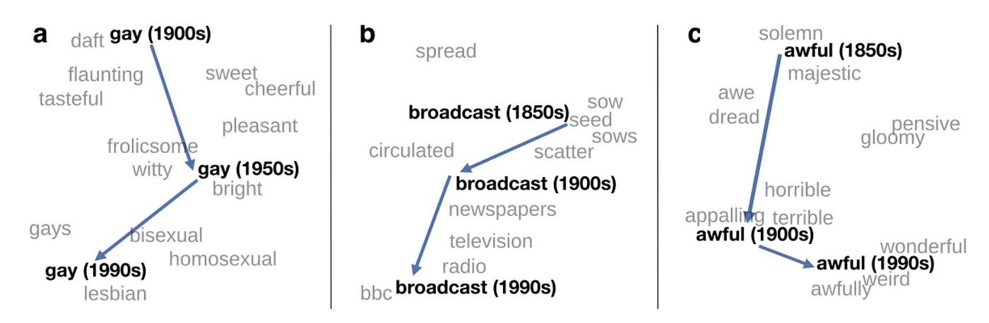From the paper written by Hamilton et al. (2016), “Diachronic Word Embeddings Reveal Statistical Laws of Semantic Change.” Link to paper here.

What are temporal word embeddings?

It has recently become popular to represent words using neural word embeddings, or those trained using neural network language modeling methods. In such cases, a dense vector is learned for each word by training on a large corpus of texts. Neural word embeddings extend the idea of distributional semantics, as the vector representation of each word is based on the distribution of its contextual words.

Given that a corpus of interest contains documents associated with a timestamp, the corpus can be divided into time periods of varying granularity: decades, years, months, weeks, days, or, sometimes, even hours. This all depends on the context of the dataset and the project. Word embeddings are trained for each subcorpus corresponding with the chosen time period. These embeddings are referred to as temporal word embeddings (also referred to as diachronic word embeddings or dynamic word embeddings).

This article will focus on Word2Vec, as it is fast to train and cheap in terms of disk space and memory consumption (Levy, Goldberg, & Dagan, 2015). Further, Word2Vec is a popular method for measuring semantic change, having been used in many influential research papers (either as the focus of the research or as a benchmark for comparison).

There is a myriad of other methods for training temporal word embeddings which will not be the focus of this article. For example, other word embeddings, such as GloVe and FastText, can be used in a similar way to measure semantic change. Packages such as Compass-aligned Distributional Embeddings make it easy to train your own aligned temporal embeddings (based on Word2Vec). Transformer-based models, such as BERT, have also been used to trace temporality in large text corpora. Evaluating a more comprehensive list of temporal word embeddings is beyond the scope of this article; for a more complete list, the reader is advised to consult the surveys conducted by Kutuzov et al., (2018) or Tahmasebi et al., (2019).

Measuring Change using Temporal Word Embeddings

Recall that each word corresponds to a dense vector representation, which is learned by training on a large corpus of text. The cosine similarity can be calculated for a word at one time period and the same word at the next time period to measure semantic change. Montariol (2021) describes two measures that can be used to track semantic change over time:

1. Inceptive drift, which computes the change of a word compared to that word at time t=0
2. Incremental drift, which computes the change of a word from one time slice to the next

The cosine similarity can also be calculated between two words of interest to see how the two words change over time in relation to each other. For example, in the paper “Diffusion-based Temporal Word Embeddings” (Farhan et al., 2020), the authors show the cosine similarity of the word “COVID” to each of four words (china, epidemic, pandemic, patients) over several months in 2020. This method allows the researcher to visualize trends such as how one word’s similarity to other keywords change over time. It is important to note that this requires you as the researcher to have a list of words of interest ahead of time.

Training Temporal Word Embeddings

Neural word embeddings (such as Word2Vec) trained independently on different temporal corpora cannot be compared directly. The vector spaces learned for each time slice are different — that is, models trained on the same data could result in vector spaces with the same nearest neighbors but different coordinates (Kulkarni et al., 2014). This is due to the stochastic aspect of the training process arising from random initialization of word vectors as well as from the order in which documents are processed (Hellrich & Hahn, 2016). Therefore, in order to ensure two vector spaces are comparable, they must be aligned via a unified coordinate system.

Note that for count-based embeddings such as PPMI (Positive Pointwise Mutual Information), alignment is not necessary, as the intersection of co-occurrence matrices of all time slices can be directly compared. The alignment is usually done by mapping all embedding spaces into a common vector space using linear transformations. One of the most popular methods of aligning vector spaces is to use orthogonal Procrustes analysis to learn a linear mapping between two embedding spaces, first introduced by Hamilton et al., 2016. Using orthogonal Procrustes to align embedding spaces is still a popular method, and the code and project is publicly available.

However, research has also shown instability may come from aligning temporal word embeddings. While orthogonal Procrustes is one of the most commonly used methods to align temporal embeddings (Gonen, Jawahar, Seddah, & Goldberg, 2020; Montariol, 2021), it is susceptible to a number of limitations. First, it is a complex alignment procedure and errors may be introduced in the process. Second, the method requires aligning the embedding spaces using the intersection of the vocabulary among all embedding spaces, which means that new words arising at a later time point cannot be compared. Finally, the procedure requires a large amount of training data, which may not be available for all corposes (Dubossarsky, Weinshall, & Grossman, 2017).

Stability of Word Embeddings

In addition to instability in methods used to align word embeddings via linear transformations, researchers have called into question the stability and fragility of word embedding models in general. Stability and consistency of word embedding models can be measured, for example, by varying different hyperparameters. Hellrich and Hahn (2016) evaluate word embeddings’ reliability, measured by the intersection of top-N nearest neighbors across several identically-parameterized Word2Vec models. The authors find that reliability is dependent on the number of epochs a model is trained for. Further, based on their finding that models trained with identical hyperparamters yield inconsistent nearest neighbors, they suggest training several identically parameterized models and combining them into an ensemble to ensure robust results. Pierrejean and Tanguy (2018) varied other hyperparameters such as architecture (i.e., CBOW and SGNS), corpus, context window size, and embedding dimension size, finding that there is large variation in nearest neighbors of the same words in different embedding spaces.

Antoniak and Mimno (2018) highlight the fragility of word embeddings by showing their sensitivity to small changes to variables such document order, corpus size, and random seeds. The authors train 50 models each for four different embedding models on different document sizes and corpora. Models are trained on three settings of document order: fixed (documents in original order), shuffled (documents in random order), and bootstrapped(documents sampled with replacement). Jaccard similarity is used to compare the top-N nearest neighbors for models trained with each combination of congurations. Jaccard similarity measures the proportion of items shared between two sets. The Jaccard similarity of two sets A and B is calculated as follows:

Antoniak and Mimno (2018) find a great deal of variability in word embedding models in terms of a target word’s top nearest neighbors as well as its rank — that is, the order in which a word appears as the nearest neighbor of the target word. This variability increases for bootstrapped documents, as this magnifies the effect of “bursty” words — those that are locally frequent but globally rare. The authors conclude that due to this large variance, embeddings do not offer an objective view of language or a corpus, suggesting future research to average results over multiple bootstrapped models.

As one solution, Gonen et al. (2020) suggest an alternative way of measuring temporal change without aligning separate embeddings, which they claim can be unstable and less reliable. The authors suggest using nearest neighbors as proxy for meaning. The semantic change is measured using the intersection of top-N nearest neighbors between words trained on different temporal corpora. This metric is used across several runs of the same word embedding algorithm and is able to detect semantic change with high stability. The authors suggest using this simpler method of comparing temporal word embeddings, as it is more interpretable and stable than using the common orthogonal Procrustes method for temporal alignment.

A Simple Experiment

As shown above, while it is necessary to align temporal embeddings trained on neural methods such as Word2Vec in order to compare them directly, doing so many introduce instability. One soultion around this was to use simpler methods of measuring change. Rather than aligning and using cosine similarity to compare words across different embedding spaces, an alternative method was to measure the Jaccard similarity of the sets of nearest neighbors for a word at two different time points.

Further, training word embeddings themselves may introduce fragility. Training just one word embedding per time slice may capture meaningful change but also introduce a lot of noise. One solution, suggested by several researchers, was to train many models and average the results, creating an ensemble of models. Further, the training documents can be shuffled or bootstrapped to introduce more robustness into the training process.

Here, I’ll walk through the steps to design the simplest of experiments for training temporal word embeddings.

1. Collect your text corpora. Clean your text as you would for any NLP project then determine into which time intervals you want to divide your text. This could be anything ranging from decades to days, depending on your data. You also want to make sure that you have enough data to train models for each time interval. For example, if you only have tens or hundreds of documents per day, perhaps you might want to expand your time window to one week or month.
2. Pick your word embedding model of choice. Word2Vec with SGNS might be the easiest to start off with — Gensim is quite easy for training models.
3. Train multiple (>50) models for each timestamped subcorpora. You can experiment with varying the hyperparameters for each run of the model: the random seed, the number of epochs, the size of the context window. You can also experiment with varying the text that you use to train your models — by shuffling the order of the documents, as well as bootstrapping your documents with replacement to ensure that some documents are seen multiple times for some models and not seen at all for other models. Complete this step for each time step.
4. You can’t average the embeddings across models becasue they are not in the same embedding space, but you can look at the nearest neighbors for the same words across different embedding spaces. For example, if you have trained on a corpus of newspaper articles about the pandemic and are interested in how the word “mask” has evolved over time, you can determine the top 50 nearest neighbors for the word “mask” for each model, then calculate the Jaccard similarity across these nearest neighbors. Higher similarity scores would indicate greater stability — despite all of the tweaking of hyperparameters and training documents, the vector representation learned for the word “mask” is quite consistent. Lower similarity scores would indicate lower stability. Complete this step across allmodels in each time step.
5. Pick a threshold (could be for each time step, could be for each keyword you’re interested in) to determine which words as nearest neighbors are stable for each time step. For example, you can determine that if words appear as a nearest neighbor of “mask” 95% of the time during one time step, then those words are considered “stable” nearest neighbors. Complete this step across all models in each time step.
6. Taking the stable nearest neighbors for each time step, compute the Jaccard similarity scores for the sets. This will indicate how much the nearest neighbors for one word changes across the time axis. You can complete this process for as many different keywords that you are interested in.
7. Alternatively, you can create a set of keywords of interest and look at the Jaccard similarity of those nearest neighbors for each time step to generate your own metric. You can track that metric over time to determine at which time points the similarity measure dips or rises.

These are just suggestions for getting started. You might want to know the relationship between stability of nearest neighbors and frequency of that word. You could be interested in how words in general have changed, and depending on your corpus, you can tweak the threshold for determine stable nearest neighbors. You could also be interested in looking at what words are unstable. For example, if a word shows up as a nearest neighbor of “mask” with very high cosine similarity but only 30% of the time, perhaps that word was used in a very specific (but not general) situation. Such investigations would depend on whether you are interested in how words changed over time in general, or in interesting and specific cases of how words were used.

Conclusion

This article attempted to explain what temporal word embeddings are and how they can be used to track semantic change over time. Concerns were discussed regarding the stability of word embeddings and common methods to align different embedding spaces. The steps for designing a simple experiment were described, and potential avenues for future projects were discussed. Temporal word embeddings are an exciting area of research within NLP and are currently being used in many different subfields. I hope that this introduction helped to explain some of these concepts.

==========

References

Antoniak, M., & Mimno, D. (2018). Evaluating the Stability of Embedding-based Word Similarities. Transactions of the Association for Computational Linguistics, 6 , 107-119.

Bloomeld, L. (1933). Language. Oxford, England: Holt. (Pages: 573).

Dubossarsky, H., Weinshall, D., & Grossman, E. (2017, September). Outta Control: Laws of Semantic Change and Inherent Biases in Word Representation Models. In Proceedings of the 2017 Conference on Empirical Methods in Natural Language Processing (pp. 1136-1145).

Farhan, A., Barranco, R. C., Hossain, M. S., & Akbar, M. (2020). Diffusion-based Temporal Word Embeddings.

Firth, J. (1957). A Synopsis of Linguistic Theory 1930–1955. Oxford.

Gonen, H., Jawahar, G., Seddah, D., & Goldberg, Y. (2020). Simple, Interpretable and Stable Method for Detecting Words with Usage Change across Corpora. In ACL. doi: 10.18653/v1/2020.acl-main.51.

Hamilton, W. L., Leskovec, J., & Jurafsky, D. (2016, August). Diachronic Word Embeddings Reveal Statistical Laws of Semantic Change. In Proceedings of the 54th Annual Meeting of the Association for Computational Linguistics (Volume 1: Long Papers) (pp. 1489–1501). Berlin, Germany: Association for Computational Linguistics.

Hellrich, J., & Hahn, U. (2016, December). Bad Company|Neighborhoods in Neural Embedding Spaces Considered Harmful. In Proceedings of COLING 2016, the 26th International Conference on Computational Linguistics: Technical Papers (pp. 2785-2796). Osaka, Japan: The COLING 2016 Organizing Committee.

Heyer, G., Holz, F., & Teresniak, S. (2009). Change of Topics over Time — Tracking Topics by their Change of Meaning. (Pages: 228)

Hilpert, M., & Gries, S. T. (2009). Assessing frequency changes in multistage diachronic corpora: Applications for historical corpus linguistics and the study of language acquisition. Literary and Linguistic Computing, 24 (4), 385-401.

Kulkarni, V., Al-Rfou, R., Perozzi, B., & Skiena, S. (2014, November). Statistically Significant Detection of Linguistic Change. arXiv:1411.3315 [cs].

Kutuzov, A., Ovrelid, L., Szymanski, T., & Velldal, E. (2018, August). Diachronic word embeddings and semantic shifts: a survey. In Proceedings of the 27th International Conference on Computational Linguistics (pp. 1384-1397). Santa Fe, New Mexico, USA: Association for Computational Linguistics.

Levy, O., Goldberg, Y., & Dagan, I. (2015). Improving Distributional Similarity with Lessons Learned from Word Embeddings. Transactions of the Association for Computational Linguistics, 3, 211–225.

Martinc, M., Montariol, S., Zosa, E., & Pivovarova, L. (2020, April). Capturing Evolution in Word Usage: Just Add More Clusters? Companion Proceedings of the Web Conference 2020, 343–349.

Montariol, S. (2021). Models of diachronic semantic change using word embeddings (Doctoral dissertation, Universit_e Paris-Saclay).

Pierrejean, B., & Tanguy, L. (2018, June). Towards Qualitative Word Embeddings Evaluation: Measuring Neighbors Variation. In Proceedings of the 2018 Conference of the North American Chapter of the Association for Computational Linguistics: Student Research Workshop (pp. 32-39). New Orleans, Louisiana, USA: Association for Computational Linguistics.

Tahmasebi, N., Borin, L., & Jatowt, A. (2019, March). Survey of Computational Approaches to Lexical Semantic Change. arXiv:1811.06278 [cs].